Inside a Transformer: A Worklog

This is currently purely a worklog in progress. Things are not formatted yet.

On residual stream as a communication channel

Residual stream?

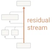
Lots about transformer layers (or blocks) & how information flows through them like a ‘stream’, as if different students in a class were given a topic to write an essay about on a long whiteboard & each student writes something new + reads what was written before

Matters mainly for ‘reading’ and ‘writing’: reading the previous layers’ outputs, and writing one’s output (which also happens to be the output from that nth layer added to the previous layers’ outputs)

block 0 -> output -> fed to block 1 -> output (enriched with its own + block 0’s info) -> fed to block 3…

this is a residual stream

reading = mainly Q @ K^T

writing = x = x + attn_output

Inside the attention sub-layer: the mechanics

Note on sub_layer: I believe this is the term the original Transformer uses to call its said block’s primary sections. For instance, the encoder has 2 sub-layers: the multihead self-attention (MHA) layer and the the FFN (or MLP) layer.

I used to understand the steps involved in the attention sub-layer, but never really got around to understanding the “how” and “why” of it.

My knowledge of the MHA mechanism, until I went deep into this, was mostly the following steps:

# assumptions
batch = 1
seqlen = 3
d_model = 32
d_head = 8
assert d_model % d_head == 0
heads = d_model // d_head

1. Initialize the weights for the incoming input x (input = also understood as the residual stream up till that point)

# assuming this already has the embeddings + positional encodings
x = torch.randn(batch, seqlen, d_model)
print(x.shape) # [1, 3, 32]

W_Q = torch.randn(d_model, d_model) # [32, 32]
W_K = torch.randn(d_model, d_model) # [32, 32]
W_V = torch.randn(d_model, d_model) # [32, 32]
W_O = torch.randn(d_model, d_model) # [32, 32]

2. Compute the query, key, and value vectors and split them into heads.

q = (x.__matmul__(W_Q)).view(batch, seqlen, heads, d_head).transpose(1, 2)
k = (x.__matmul__(W_K)).view(batch, seqlen, heads, d_head).transpose(1, 2)
v = (x.__matmul__(W_V)).view(batch, seqlen, heads, d_head).transpose(1, 2)
q.shape, k.shape, v.shape # [1, 4, 3, 8], [1, 4, 3, 8], [1, 4, 3, 8]

3. Compute the attention scores

attn_scores = q.__matmul__(torch.transpose(k, -2, -1))
attn_scores.shape # [1, 4, 3, 3]

mask should also be applied in case of an attention inside the decoder, omitting for now (sample masking is done later here)

4. Compute the attention weights

attn_weights = torch.softmax(attn_scores / d_head ** 0.5, dim=-1)
attn_weights.shape # [1, 4, 3, 3]

5. Compute the attended values

attended_vals = attn_weights.__matmul__(v)
attended_vals.shape # [1, 4, 3, 8]

6. Combine the split heads back into the original dimension

output_heads_combined = attended_vals.transpose(1, 2).contiguous().view(batch, seqlen, d_model)
output_heads_combined.shape # [1, 3, 32]

7. Compute the output projection

output_proj = output_heads_combined.__matmul__(W_O)
output_proj.shape # [1, 3, 32]

But what is the intuition behind these steps? What is the best way of understanding the “how” and “why” of these steps? A few specific questions:

• What is the attention weight trying to tell us?
• There are batches of tokens that are being processed in parallel to get the output (input + output_proj, i.e., the updated “residual stream”) from the MHA sub-layer of the transformer. How do I exactly visualize this? What happens sequentially? What happens in parallel?
• Why do we need the output projection? What is the intuition behind it?

Trying to gain some deeper intuition

The Anthropic paper[1] suggests that we break down the MHA sub-layer into 2 “circuits”: the QK circuit and the OV circuit.

The following is a set of calculations that I did (once again), step-by-step, to gain some deeper intuition.

1. Initializing some initial initializables

For this, I will assume the input is: “The cat sat”. I will also assume the d_model = 8, and d_q[-1] = 4.

torch.manual_seed(42)
seqlen = 3 # because the input is "The cat sat"
attn_scores = torch.randn(seqlen, seqlen) # randomly initializing for the sake of quick testing
d_hidden = 8 # aka d_model
q_last_layer = 4 # aka d_q[-1]

2. Masking, softmaxing, and getting the attention weights (not going to do head splitting here for the sake of simplicity)

upper_triangular = torch.triu(torch.ones_like(attn_scores), 1)
mask_bool = upper_triangular.bool()[:, :]
attn_scores_w_causal_mask = torch.masked_fill(attn_scores, mask_bool, value=torch.tensor(float("-inf")))
attn_w = torch.softmax(attn_scores_w_causal_mask / q_last_layer ** 0.5, -1)
attn_scores_w_causal_mask, attn_scores, attn_w

This gives us:

# attn_scores_w_causal_mask
tensor([[ 0.3367,    -inf,    -inf],
         [ 0.2303, -1.1229,    -inf],
         [ 2.2082, -0.6380,  0.4617]]),

 # attn_scores
 tensor([[ 0.3367,  0.1288,  0.2345],
         [ 0.2303, -1.1229, -0.1863],
         [ 2.2082, -0.6380,  0.4617]]),

 # attn_w
 tensor([[1.0000, 0.0000, 0.0000],
         [0.6630, 0.3370, 0.0000],
         [0.6029, 0.1453, 0.2518]])

The following are assumed to be the attention scores, attention scores (with masking), and attention weights for the input “The cat sat”.

(tensor([[ 0.3367,    -inf,    -inf],
         [ 0.2303, -1.1229,    -inf],
         [ 2.2082, -0.6380,  0.4617]]),

 tensor([[ 0.3367,  0.1288,  0.2345],
         [ 0.2303, -1.1229, -0.1863],
         [ 2.2082, -0.6380,  0.4617]]),

 tensor([[1.0000, 0.0000, 0.0000],
         [0.6630, 0.3370, 0.0000],
         [0.6029, 0.1453, 0.2518]]))

Looking at the 3x3 attention weights matrix, I can picture this as:

1. to understand “cat”, how much will I have to look at the token “the”? —> exactly 1.000, so strong relevance for this computation.
2. to understand “sat”, how much will I have to look at the token “the”? —> 0.6029, so a pretty solid relevance for this computation.
3. to understand “sat”, how much will I have to look at the token “cat”? —> 0.1453, so an okay-ish relevance, not as strong as the one just before.

3. Computing the attended values

# assuming:
X_IN = torch.randn(seqlen, d_hidden) # [3, 8]
W_V_ = torch.randn(d_hidden, d_hidden)
V = X_IN.__matmul__(W_V_)
W_O_ = torch.randn(d_hidden, d_hidden)
ATTENDED = attn_w.__matmul__(V)
print(f"""W_V: {W_V_.shape} # [8, 8]
{W_V_}

V: {V.shape} # [3, 8]
{V}

attended weights: {ATTENDED.shape} # [3, 8]
{ATTENDED}
""")

# which gives us something like:
W_V: torch.Size([8, 8])
tensor([[ 0.0349,  0.3211,  1.5736, -0.8455,  1.3123,  0.6872, -1.0892, -0.3553],
        [-1.4181,  0.8963,  0.0499,  2.2667,  1.1790, -0.4345, -1.3864, -1.2862],
        [-0.8371, -0.9224,  1.8113,  0.1606,  0.3672,  0.1754,  1.3852, -0.4459],
        [-1.2024,  0.7078, -1.0759,  0.5357,  1.1754,  0.5612, -0.4527, -0.7718],
        [ 0.1453,  0.2311,  0.0087, -0.1423,  0.1971, -1.1441,  0.3383,  1.6992],
        [ 2.8140,  0.3598, -0.0898,  0.4584, -0.5644,  1.0563, -1.4692,  1.4332],
        [ 0.7281, -0.7106, -0.6021,  0.9604,  0.4048, -1.3543, -0.4976,  0.4747],
        [-0.1976,  1.2683,  1.2243,  0.0981,  1.7423, -1.3527,  0.2191,  0.5526]])

V: torch.Size([3, 8])
tensor([[-3.3538, -2.6614,  5.1813, -0.1024,  0.1555, -0.1970, -0.2466, -2.8980],
        [-0.4393,  1.2727,  0.4840, -3.8536, -1.8261,  5.3907,  0.3668, -2.1857],
        [-0.3070, -0.7861,  2.5214, -1.5471, -1.1485,  1.0364,  2.6574, -0.5662]])

attended weights: torch.Size([3, 8])
tensor([[-3.3538, -2.6614,  5.1813, -0.1024,  0.1555, -0.1970, -0.2466, -2.8980],
        [-2.3715, -1.3356,  3.5982, -1.3666, -0.5123,  1.6862, -0.0399, -2.6579],
        [-2.1632, -1.6177,  3.8292, -1.0111, -0.4607,  0.9254,  0.5737, -2.2074]])

4. Computing the output projection

OUTPUT_PROJECTION = ATTENDED.__matmul__(W_O_)
print(f"""{OUTPUT_PROJECTION.shape}
{OUTPUT_PROJECTION}""")

# which gives us something like:
torch.Size([3, 8])
tensor([[ 10.8347,  -4.9027,   7.4389,  -2.5553,   9.3776,  -2.1711, -14.9518,
          -5.0850],
        [  8.7450,  -3.9095,   3.6260,  -2.4063,   5.4063,  -1.0348, -11.8651,
          -2.1552],
        [  9.2331,  -4.1688,   2.8769,  -2.0400,   4.9977,  -1.7839, -11.5206,
          -2.4551]])

5. Combining the attended values and the output projection for the updated residual stream

residual_stream = X_IN + OUTPUT_PROJECTION
# this is bascially:
#   x_in + attended_val @ W_O {here, x_in = (enbeddings + pos_encodings), and attended_val @ W_O = output_projection}
# = x_in + (attention_weights @ V) @ W_O
# = x_in + ((Q @ K.T) @ (x_in @ W_V) @ W_O) {simplifying the attn weights a little here, softmax and being divide by d_k ** 0.5 are omitted}
residual_stream.shape, residual_stream

# which gives us something like:
(torch.Size([3, 8]),
 tensor([[ 12.7616,  -3.4154,   8.3396,  -4.6608,  10.0561,  -3.4056, -14.9948,
           -6.6897],
         [  9.1009,  -4.5961,   3.1327,  -2.1649,   4.2954,  -0.9433, -14.1820,
           -2.3720],
         [  8.9234,  -4.5645,   3.6803,  -2.6616,   4.4057,  -1.8470, -12.3491,
           -2.1242]]))

and that’s the output from the MHA sub-layer of the transformer.

A little more intuition on what this means

For, say, the word “sat” (3rd word in the sequence):

W_sat = residual_stream[2]

This is:

residual["sat"] aka residual[2]
= x_in["sat"] + attended_val["sat"] @ W_O

Let’s assume our attention weight matrix was:

This means:

attention_weights["sat"] = [0,20, 0.50, 0.30]

So, residual["sat"] is:

=> x_in["sat"] + (attention_weights["sat"] @ V) @ W_O
=> x_in["sat"] + ([0.2, 0.5, 0.3] @ [V_The, V_cat, V_sat]) @ W_O
=> x_in["sat"] + (0.2 * V_The + 0.5 * V_cat + 0.3 * V_sat) @ W_O
=> x_in["sat"] + (0.2 * x_in["the"] + 0.5 * x_in["cat"] + 0.3 * x_in["sat"]) @ W_O

Hence W_sat is:

x_in["sat"] + (0.2 * x_in["the"] + 0.5 * x_in["cat"] + 0.3 * x_in["sat"]) @ W_O

So basically…

We can divide this process into 2 parts:

1. the QK circuit
2. the OV circuit

# the QK circuit:
Q @ K.T
=> (x @ W_Q) @ (x @ W_K).T

# the OV circuit:
(attention_weight @ V) @ W_O
=> (attention_weight @ (x @ W_V) @ W_O)
=> (attention_weight @ x) @ (W_V @ W_O)

Why talk about W_OV = W_V @ W_O? => For analysis and interpretability

Instead of thinking “first we transform by W_V, then later by W_O,” we can think: “This attention head applies a single combined transformation W_OV to move information.”

Update on the questions I asked myself earlier

1. What is the attention weight trying to tell us?
   => I know now how to think about it.
2. There are batches of tokens that are being processed in parallel to get the output (input + output_proj, i.e., the updated “residual stream”) from the MHA sub-layer of the transformer. How do I exactly visualize this? What happens sequentially? What happens in parallel?
   => Need to get my head around this. I’m sure this is much simpler than I’m making it out to be. Will update this soon.
3. Why do we need the output projection? What is the intuition behind it?
   => This is basically how much to move the information forward based on the attention weights. Will update more details on this to come.

Still lots of questions to answer. Will update this as I go along.